Account Balances 2
By Richard Rost

 3 years ago
Track Account Balances & Transactions, Part 2
This is part 2 of my Microsoft Excel tutorial series where I teach you how to track your account balances and daily transactions. We'll be using basic formulas, math equations, conditional formatting, tables, and the SUMIFS function.
Prerequisites
Dedication
- Dedicated to my fiance, Lauren ❤️🐧
Members
There is no extended cut, but here's my workbook file:
Silver Members and up get access to view Extended Cut videos, when available. Gold Members can download the files from class plus get access to the Code Vault. If you're not a member, Join Today!
Recommended Courses
Want More Excel?
Most of what I do is Microsoft Access, so if if you want to see me post more Excel videos, make sure to comment below: "I want more Excel!"
Keywords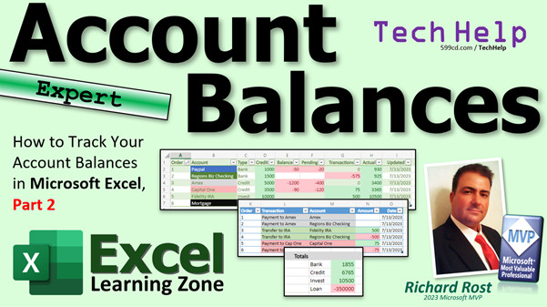
excel 2021, excel 2016, excel 2019, excel 365, microsoft excel, ms excel, ms excel tutorial, #msexcel, #microsoftexcel, #help, #howto, #tutorial, #learn, #lesson, #training, #database, #techhelp, track microsoft excel account balances, personal finances, daily spending transactions, track finances, balance chart, credit and debit, banking activity, credit card balances
Intro In this video, we continue working with account balances in Microsoft Excel, building on the foundation set in part one. I will show you how to save your workbook, color code accounts for better organization, use the format painter to quickly apply formatting, and set up conditional formatting to highlight positive and negative values. We'll also cover converting your data to tables for easier sorting and filtering, inserting rows, using the SUMIFS function to total account types, and maintaining formatting as you update your records. This is part 2.Transcript This is part two of my account balances and Excel series. So if you have not watched part one yet, go watch part one first. What are you doing here? Go watch part one. Go beat it. Scram. Here is a link. You will find it on my YouTube channel. You will find it on my website. It is free. You will find a link down below you can click on. So go watch that and come on back.
So here we are back in our sheet and we are continuing on from yesterday. First thing we are going to do is save our work because I forgot to save it in the last video. So click here where it says book one and we will just type in account balances. Then presenter. There you go. That is it. It is saved. It is in your one drive. That is the default location. If you want to browse your one drive, click right here. It will take you through browsing all that, but you do not have to do that right now.
When you are working with the online version and with the local version, too, this auto save feature happens every so often, but it is still a good idea to manually save your work once in a while.
Next up, I like to personally color code my accounts. It just makes things easier. Plus, over here, it is easier to see, like, okay, these are MX related, this is IRA related, whatever. So, we will do PayPal. They have a blue color like that, and we will do white for the front. Regions is greenish. We will do that with white. MX, I go with the platinum color. Let's go with that. Capital One is kind of reddish. We will do them. Let's pick this, but we do not want that crazy red, so we go to more colors and lighten it up a little bit, maybe over here. That looks better. Fidelity is green, but we do not want to use the same green as that one. So we will pick a light green like that. Mortgage - because, you know, the mortgage.
Okay, so there you go. Now, what I want to do is color the stuff over here the same as over here so I can quickly, visually see. I generally do it wherever the account you are paying into is. For example, I will do these as both the MX color. These will be both the Fidelity color. Even though it is coming out of Regions checking, this is really an MX transaction. Makes it easier to see everything.
Now I do not want to have to pick those colors again because I already got them, so I am going to take this MX color and use the format painter, this guy, and paint over this stuff - just these. Makes it easy to see pairs. Then I will do the same thing with Fidelity. Here is Fidelity, format painter, and paint over these guys.
I cover the format painter and lots of other cool formatting like headers and photos, freezing panes, all that kind of stuff in Excel Beginner Level 5. Find a link to that down below. Lots of cool stuff. In this video, I am only showing you the basics, just the real quick stuff.
Now, let's say if you do another transaction, we will do five. Let's say transfer. Fill aside, ignore that. I hate that. We will do transfer to. Now, see, I typed in transfer to and that thing came up. I am going to say in here transfer to PayPal. This is going to be going into PayPal. Let's say we are transferring 150.
Then six, same thing. I do not want that. Turn that off. Pull away. Transfer to PayPal. It is coming out of Regions checking again. Minus 150. Now I want to use the format painter and paint over this stuff so I can see that is my PayPal transaction.
Just makes it easier. In the future, you want to keep copying those, because, again, you will leave these here for transactions that you use on a regular basis. For the one-off side, I might not even bother coloring, I might just leave white.
Next up is some conditional formatting. I want positive values in here to show up green and negative values to show up red. We can do that with some conditional formatting.
Now, one thing is when you start Excel, usually you get this minimized single row ribbon. I like to turn the big ribbon on for stuff like this. Go to the classic ribbon over here. You will see this thing. It looks more like the full-sized ribbon in Excel. Close it if you want to. If space is a concern, like here when I am recording videos, I have my browsers in this little tiny window because that is the size I record. I record 720p video, but on my full screen, I have a big giant monitor on my desk. I leave the big ribbon on most of the time.
Now, I have a whole separate video on conditional formatting. You can go watch this. This is a free one. I also cover it in my Excel Beginner Level 2 class. Beginner Level 2 follows Beginner Level 1. Beginner Level 1 is the free one. Level 2 is just a dollar. It is also free for all members on my YouTube channel and on my website. So if you want more information on that, let me know and I will hook you up with it.
Conditional formatting is what it says. It will format the cells conditionally, based on whatever condition you give them. Negative numbers less than zero are going to be red. Positive numbers greater than zero will be green. Zero, we will just leave alone.
Highlight these cells right here. Conditional Formatting. We are going to pick Highlight Cells Rules and then Greater Than. That is going to open up this guy. Now, it opens up a window in the desktop version of Excel, but this online version opens up this pane over here. The range D2 to H7, that is fine.
Highlight Cells With, that is going to be Cell Value greater than, and in here, put zero. Now, right here you can change the format. Just drop this down and green, this one right here. There are already some preformatted formats in here. I like this green and this red. So we'll pick this green. You can change it more if you want to, with the colors and stuff right here.
Now I am going to hit Done and look at that. You can see over here all the positive values are now green. But hold on, we are not done. We are going to add another value right there, new rule. Cell value less than zero. We are going to leave that red one here now this time. Then hit Done. There you go. Close that. There is your conditional formatting. Super easy to do.
While we are at it, I want to format these as well. Now, I do not want to go through the steps again, so what will I use? The format painter. Pick any one of these cells, click on the format painter, then paint over this region here. There you go. Now here are your pluses and minuses, super sweet here.
I forgot some alignment over here. Click on this one. We are going to right align that one. Actually, no, we are going to left align that one. We are going to right align - there we go.
Next up, we are going to turn each of these sections into what are called tables. Tables have a lot of benefits. I covered tables in detail in my Excel Beginner Level 4 class, working with data tables. There are a lot of benefits with tables.
For example, in the old days, if you wanted to sort something, let us say you wanted to sort by credit or the actual balance, whatever, if you just sorted this, picked sort, it would literally just sort that column and everything else would get scrambled. That is not so much a problem anymore, because Excel has gotten a lot smarter and it can see that that is kind of a table right there.
There are a lot of other benefits too. For example, inserting rows. Let us say you wanted to insert something above Capital One. If I insert a row here, right click, insert a row, what did I just do? Well, I inserted it over here. I also inserted a row over here. It is one big row. Excel does not see a difference. I am going to undo that, Control-Z.
Basically, tables allow you to insert and delete rows in just that area that you have marked as a table. They are real easy to set up. All you do is select the outer boundary of your table, go Format as Table, and then pick a style. I am going to go with this one.
OK, Format as Table, A1:I7, that seems about right. Table has headers, yep, that is the header row, and then hit OK. There you go. It expands a little bit. Also, what it does is it gives you these little drop down boxes here. So now you can filter and sort based on the data in that table.
You can do a quick sort there. Or you can come over here and say, I want to filter it. I only want to see bank items, hit apply. The data is still there, it is just filtered. If you want to remove that filter, drop that down, and then select all, then hit apply. There you go. I will go back to your original custom sort. This is why I like the custom sort over here. Drop that down. Sort smallest to largest. Now I am back to my way I like to see them.
Now we can treat this guy as a table over here as well. Format as table. Pick, let us do the blue one. There. I am going to get rid of that custom color that I put up here before by just dropping this down and picking no fill. That way you get whatever the default was for that particular table style. I cover styles in one of my future classes as well. Looks like that is Beginner 3.
I used to have to say in the old days, "well, I will cover that in a future class." Now I have got all those classes recorded, so now I can just tell you, if you want to learn more about it, go here. That was the biggest complaint in the surveys that people used to fill out when I first started doing this. I cannot teach you everything at once. I have to spread it out because that is how the brain works.
But now if you want to insert a row somewhere, you can just come here, right click, and then go Insert Table Rows Above. Look at that. It inserts it just here for you. Now, if you want, you can put in here - here is what I like to do with sorting. Let us say I added a Regions account. I will make this three. This could be Regions saving, let us say bank. Maybe I have 2,000 in there.
Notice all of your conditional formatting and stuff will copy down, too, because this is a table. Now these are one, two, three. I want to keep that numbering going. So now, I am going to select one, two, three, and I am going to click this guy, the autofill handle, drag it down, and they will get renumbered, four, five, six, seven. I still keep my custom order there.
That is important. When I inserted that row, it did not insert it into this table, because it is two separate entities. Sometimes you want that. Sometimes you want things on different sheets. Sometimes you want to see them side by side. Like I said last video, this is something I like to see side by side.
A little side note - if you are planning on eventually upgrading from Excel to Access, as a lot of people do, if you have your data in Excel in tables, it becomes a lot easier to move up to Access, too. There are just some benefits there.
How about some totals down here on the bottom for our different types of accounts? I want to see what the total is for my bank accounts, my credit accounts, my investment accounts. So I will come down here and let us go totals. I am going to copy each one of the types of accounts. We got bank, put bank there, or you could put it the same way - that is my bank. We got credit. We got investment, loan, just copying and pasting those down there.
Now I see it brought in the table format with that, so I do not like that that brought that green down with it, see, because there is a format on there. I am going to click on a blank cell. I am going to hit the format painter and just paint over those and it will get rid of that.
That happened to be a right justified cell, so we will make that go back to left, but it gets rid of the outlining.
Here I want to put the total of the actual amount if this is the right column that says bank in it. Again, we are going to go back to our SUMIFS function: =SUMIFS.
What is the sum range? I am going to click slow, so I can show, so I can see it. The sum range is this range right here. Now notice something happened. When I selected that, instead of getting the whole column, which you do not want to do with the table, look there, it says Table1[Actual]. This is Table1 - Excel named it, and it uses the column header Actual. That is pretty cool.
Now hit comma, what is the criteria range, the list of criteria? That is over here. Table1[Type], comma, and what value in that criteria range am I looking for? I am looking for bank. Close it up, press enter, and look at that - 3980 for these three bank accounts. 2,000, 3,980. That seems about right. If you select these, it will tell you down here sum 3980.
Now we can autofill this down. There you go. Maybe a little conditional formatting, format paste, click and drag. Boom. There you go. Make this gray, I do not know. Give it something to differentiate it. Let's go. All right. Cool. Put a box around this if you want to. There are all kinds of stuff you can do. There are your totals.
Now, this new conditional format, since we changed to tables, and I conditional format, SUMIFS, excuse me, let us change our SUMIFS in here because this is still using the old, the complete column. Let us change that. So let us get rid of this. So this is N, which is over here, then M, then B2. Let us change this. So we are going to select all that, delete. We are going to select: what is the sum range? The sum range is here. Notice it changed Table to Amount. That is Table2 over there on that side. Comma. The criteria range is the account right there. Comma. The value we are looking for is that guy. Close it up, press enter.
Notice now it changed. Did not get it right the whole way - I messed it up. Oh, that is my bad. I picked Type. Good thing I made that mistake. I will leave that in there for you to see. Sometimes if I make a mistake in a video, chances are you might make that same mistake. I like to leave those mistakes in the video. That was just careless typing. Careless picking of cells. So this should not be the Type, this should be the Account right there. I can close that. Enter. There you go. 150, 650 looks about right. Notice every cell in that entire column was updated, because that is how tables work also.
If you want to add something else over here, just type in the row right below the table and it will expand the table for you. Put a 7 in there. Tab. Notice how the border around that table expanded. Payment to Cap One. Where is it going to? Capital One, copy, paste. How much? What did we have? 40 bucks at the end of this? I had, so 40 today. Enter.
Come back over here. We are going to go eight. Payment to Cap One. It is coming from Regions checking, and that will be minus 40. Now I am going to format paint the Capital One colors over this whole area here. I know that is Capital One stuff. Notice that conditional formatting came down for us automatically because it sees it is a table.
Got a mortgage payment. We will do nine. We will do ten. We will do them at the same time. We will do a mortgage payment. Mortgage payment. It is going to go into the mortgage, and it is coming out of Regions savings this time.
Again, you should get in the habit of copying and pasting and not typing, unless you are really simple. The mortgage color is that, and we will do this. We will say this was, I do not know.
Now you can easily see what is going on over here. You can already see I made that payment, it has not posted yet. You are looking at your savings account balance and you say, oh, wait a minute, I have a problem. This is the column you want to be looking at to make sure nothing is in the red over here. In fact, in my personal spreadsheet, I changed it so that this Actual, I changed my conditional formatting a little bit, so if this Actual goes below 500, then it will go red for under 500. I try to keep 500 as the minimum for all my accounts. So if it goes below that, it is like, oh, better do something fast.
If you like this stuff and you want to learn more, again, if you have not watched my Excel Beginner 1 class, it is free. Go watch that. Beginner 2 covers autofill. Three and four have lots of great stuff in them. Tables in Beginner 4. SUMIFS is in Expert 5. We have drop-down lists in Expert 10, all kinds of stuff.
I have lots of Excel classes. I have five beginner classes and I have 11 expert classes. I am currently in the process of rerecording all of these for the latest version. It is currently 2023. All the stuff that I cover in these older versions work just fine. Excel really has not changed much. They have added some new stuff to it. I have separate videos for the things they have added. Like, when they added XLOOKUP, I made this lesson. XLOOKUPs are really cool. All the older stuff is still just fine. They have been using it for 30 years and not a lot of the stuff changes. Pivot tables and the financial functions and dates and times. All the stuff is all the same. They cannot change it because they are going to make everybody mad. So if you learned something in 1996, chances are it still works today in Excel.
Tomorrow, in tomorrow's video, we are going to start building the same exact thing in Microsoft Access for those of you who are Access folks. It is good to learn how to do it in Excel too, because if you want to teach someone else - like I had to teach Lauren how to do this. You can watch this if you have to teach some of your coworkers or your mom or someone how to basically track their finances in Excel. This is much easier for people who do not want to be computer gurus.
Since I know most of my students are Excel nerds, we are going to be doing this tomorrow in Access and doing some additional cool things that you cannot do in Excel that you can do in Access.
If I said we are doing it in Excel earlier, I apologize.
So that is going to do it for part two of account balances. I am not going to rule out part three, but I have nothing else planned at this point except the Access stuff. So if there are things you want to see me add to this, let me know. If enough of you are interested, post comments down below. If enough of you are interested, if there is stuff you want to see or questions, maybe there will be a part three. I do not know. Squeaky wheel gets degrees. So the more times people request something, the more likely I am to take the time to record a video about it.
So there you go. There is your TechHelp video for today. I hope you learned something. Live long and prosper, my friends. I will see you next time.
How to become a member: Click the join button below the video. After you click the join button, you will see a list of all the different membership levels that are available, each with its own special perks.
Silver members and up will get access to all of my extended cut TechHelp videos, live video and chat sessions, and other perks. Gold members get access to download all of the sample spreadsheets that I build in my TechHelp videos, plus my code vault where I keep tons of different functions that I use and more. Platinum members get access to all of the previous perks, plus all of my beginner full courses and one new expert course every week. These are the full-length courses found on my website and not just for Excel. I also teach Word, Access, Visual Basic, ASP, and lots more.
Now, when you do sign up to become a member, I need you to email me and tell me "I want more Excel." The vast majority of my videos are for Microsoft Access because that has been my focus for the past few years; however, I am happy to add more Excel videos if I get more Excel members, so make your voice heard and I will make lots more TechHelp lessons for Excel.
Do not worry; these free TechHelp videos are going to keep coming. As long as you keep watching them, I will keep making more and they will always be free.Quiz Q1. What is the main reason the presenter recommends color coding account rows in the Excel sheet?
A. It makes the sheet look more colorful
B. It helps to visually distinguish different accounts quickly
C. It is required for Excel formulas to work
D. It is necessary for the auto save function to work
Q2. What is the function of the Format Painter tool in Excel as described in the video?
A. It saves your file automatically
B. It copies and applies formatting from one cell or group of cells to another
C. It inserts new rows into a table
D. It filters rows based on condition
Q3. How does the presenter suggest using conditional formatting in the account balance spreadsheet?
A. To automatically format currency symbols
B. To make positive values appear green and negative values appear red
C. To bold the header row
D. To highlight duplicate account names
Q4. What benefit does converting a data range to an Excel Table provide, according to the video?
A. It enables automatic color coding
B. It restricts editing to only one user
C. It simplifies sorting, filtering, and inserting rows within just that table
D. It increases the worksheet's maximum row limit
Q5. When adding or editing data within an Excel Table, what happens to conditional formatting and formulas?
A. They are removed and need to be reapplied manually
B. They do not extend to new rows
C. Conditional formatting and formulas automatically apply to new rows in the table
D. Conditional formatting only works on the original rows
Q6. Why is it easier to import data from Excel into Microsoft Access when using tables?
A. Tables are easier to print
B. Tables ensure data is organized in a structured way compatible with Access
C. Access only supports table data from Excel
D. Non-table data imports faster
Q7. What function is used in the video to sum values by account type, such as "Bank", "Credit", or "Investment"?
A. SUM
B. COUNTIF
C. SUMIFS
D. VLOOKUP
Q8. What happens if you insert a row inside an Excel Table?
A. The row is added only to the table, not affecting other areas
B. All rows outside the table are deleted
C. The entire worksheet is shifted
D. Only formatting, not data, is added
Q9. How does Excel refer to columns and data within a table for formulas?
A. By traditional cell references only (like A1:A10)
B. Using structured references like Table1[Actual]
C. It does not allow formulas in tables
D. Only through the column header's color
Q10. What is the effect of applying a filter to a column in an Excel Table?
A. Filters all sheets in the workbook
B. Removes all rows except the header
C. Displays only the rows that meet the selected criteria, while hiding the others
D. Deletes the filtered-out data
Q11. What best describes the use of autofill with numbers in tables, as shown in the video?
A. Autofill only works on text fields
B. Autofill can continue number sequences in a column automatically
C. Autofill changes colors instead of values
D. Autofill is not available in Excel tables
Q12. What Excel feature is used to left align, right align, or otherwise change text alignment in cells?
A. Conditional Formatting
B. Sort and Filter
C. Alignment buttons on the ribbon
D. Format Painter
Q13. According to the video, what is a convenient way to add a new row to an existing table?
A. Insert a row anywhere on the worksheet
B. Add data in the cell directly below the table and press Tab
C. Copy and paste the entire table somewhere else
D. Use the Undo command
Q14. What does the presenter recommend as a simple alert for potentially low balances?
A. Using an Excel macro to send emails
B. Conditional formatting to highlight values below a certain amount, like $500, in red
C. Setting the worksheet background to red
D. Hiding accounts with low balances
Q15. What must you do to maintain the correct formatting/coloring when adding new transactions, based on the presenter's method?
A. Repeat all conditional formatting steps manually
B. Use the format painter to apply the same format to new rows/transactions
C. Save the worksheet as a template
D. Re-enter all existing transactions
Q16. When using SUMIFS in Excel tables, why is it important to use the correct column references?
A. Incorrect references will cause an error or incorrect totals
B. SUMIFS ignores table columns
C. Any column will work, Excel is forgiving
D. SUMIFS only works outside tables
Answers: 1-B; 2-B; 3-B; 4-C; 5-C; 6-B; 7-C; 8-A; 9-B; 10-C; 11-B; 12-C; 13-B; 14-B; 15-B; 16-A
DISCLAIMER: Quiz questions are AI generated. If you find any that are wrong, don't make sense, or aren't related to the video topic at hand, then please post a comment and let me know. Thanks.Summary Today's video from the Excel Learning Zone continues our exploration of managing account balances using Excel, and this is part two of the series. If you have not yet watched part one, I strongly recommend doing so before proceeding further, as it sets the foundation for everything we will cover here. You can find that video on my website or YouTube channel for free.
Picking up from where we left off, let us first save our Excel file properly this time. Simply save your workbook as 'account balances' so it will now be stored in your OneDrive by default. Though Excel and OneDrive provide auto-save functionality, it is still good practice to save manually from time to time, both in the online and desktop versions.
Next, I like to color code accounts for a clearer overview. Assigning specific colors to each account—perhaps blue and white for PayPal, greenish hues for Regions, a platinum shade for MX, a shade of red for Capital One, and different greens for Fidelity—makes it quicker to visually identify different accounts and their related transactions. When setting up these color schemes, aim to keep similar transactions and their source or destination accounts paired with the same shade, using tools like the format painter to quickly duplicate formatting across your sheet.
Using the format painter helps avoid repetitive color selection and ensures consistency. For instance, if you have an MX transaction, use the format painter to match all MX-related rows and do the same for other accounts. For frequently used transactions, keep the formatting for quicker entry and clear organization. Occasional or one-off transactions might stay with the default white background.
Now, let us use conditional formatting so positive values display in green and negative values show up in red. This visual cue makes it much easier to spot credits and debits at a glance. You can find the conditional formatting feature on the classic Excel ribbon, which I prefer over the minimized view, especially when working on more detailed formatting tasks. If you are interested in delving deeper into formatting options, headers, photos, and features like freezing panes, check out my Excel Beginner Level 5 class, which you will find linked below.
To set up conditional formatting, highlight your range of values and create rules so that any cell with a value greater than zero turns green, and any less than zero turns red. This process works slightly differently in the web and desktop versions, but either way, you will see your sheet come alive with this helpful color coding. To replicate this formatting elsewhere on your sheet, just use the format painter.
Some alignment adjustments may be needed as well. For improved presentation, left-align or right-align your columns as appropriate.
The next concept to cover is converting these sections into tables. Tables in Excel offer a host of benefits: they make sorting and filtering easier, allow for the seamless insertion and deletion of rows within defined areas, and provide built-in styling options. By selecting your data range and using the 'Format as Table' command, you can instantly convert your data into a structured table with header recognition and filtering capabilities.
Tables also prevent the mishaps that used to occur when sorting columns independently, which could scramble your data. Now, sorting and filtering inside a table is safe and efficient. With tables, inserting new rows will only affect data within that table—not other tables or parts of your workbook.
For instance, if you add a new account such as 'Regions savings' with $2,000, Excel will recognize the addition, copy down the conditional formatting, and properly update the table numbering using the autofill feature. Just grab the handle and drag down to keep your numbering sequence intact.
Separating your data into different tables or sheets, or keeping them side by side, depends on your preference and workflow needs. An additional advantage of using tables in Excel is that they make it much easier to migrate your data to Microsoft Access later, since Access loves well-structured table data.
If you want to see totals for different account types—bank, credit, investment, loan, and so on—set up a summary row at the bottom and use Excel's SUMIFS function. While entering formulas in a table, you get the benefit of structured references, such as Table1[Actual] for the sum range, and Table1[Type] for the criteria. This keeps your formulas clean and makes copying or modifying them straightforward. Any formatting errors or misalignments you encounter are also easy to fix with the format painter or alignment tools.
If you accidentally select the wrong range in your SUMIFS or make a careless mistake, do not stress. I often leave those errors visible in the videos because chances are, you might make the same mistake, and it is helpful to see how to correct it in practice.
When you extend your tables by adding more rows, Excel automatically expands the tables, copies down formatting, and updates formulas as necessary. For more account payments, such as a new 'Payment to Cap One' or a mortgage payment, simply enter them in the next row, assign the right account, type, and amount, and reapply color coding if you wish. The conditional formatting will also extend automatically.
For critical tracking, I recommend watching out for low balances. In my personal sheet, I set up a formatting rule so any account balance dropping below $500 gets flagged in red. This can help you quickly realize when you need to make adjustments.
If you want to learn more about these techniques, be sure to check out my Excel Beginner 1 class, which is entirely free. Beginner 2 goes into autofill, levels three and four cover more intermediate topics like tables, and various expert-level courses tackle advanced tools like SUMIFS, drop-down lists, and more. I offer five beginner and eleven expert Excel classes, regularly updated for the newest versions, but all essential skills remain applicable over the years. The same classic features have worked in Excel for decades, making your learning investment worthwhile.
Tomorrow, we will begin translating this process into Microsoft Access. This is especially helpful for those interested in building more advanced or automated financial tracking solutions. Learning it in Excel is also useful if you need to teach others, such as coworkers or family members, especially those less comfortable with advanced software.
If you have suggestions for additional topics in this series or if you want to see a part three, let me know in the comments. I am always open to new ideas and feedback.
For more details and step-by-step video guidance on everything discussed here, visit my website at the link below. Live long and prosper, my friends.Topic List Saving and naming your Excel workbook
Using OneDrive for file storage
Color coding account rows for clarity
Copying cell formatting with the format painter
Applying conditional formatting for positive and negative values
Switching between minimized and classic ribbon views
Creating Excel tables from data ranges
Sorting and filtering data in Excel tables
Inserting and deleting rows within tables
Auto-filling and renumbering table columns
Using the SUMIFS function with structured table references
Copying conditional formatting to new regions
Adding totals by account type with SUMIFS
Expanding tables automatically by entering new rows
Adjusting table formatting and cell alignment |